

Digital Oscilloscope Company Shares How to Choose the Right Bandwidth for Your Lab
2026-11-18
Choosing an oscilloscope bandwidth for your lab is less about the biggest number on the datasheet and more about what your signals actually do at the probe tip. The engineers at TPS learned this across countless lab benches, and this guide turns those lessons into a practical selection process. It will help you avoid both overpaying for speed you will never use and under-specifying a scope that quietly distorts every reading.
Bandwidth starts with the fastest signal you actually probe, not the scope’s price tag
The price tag on a scope tells you very little about the bandwidth your current project actually demands. A modest clock can still have edges sharp enough to create harmonics that go well past its fundamental frequency, and those are often where ringing, overshoot, or timing problems become visible. The signal at your probe tip sets the requirement, not the badge on the front panel.
Before reaching for the high-end model, find the fastest edge you genuinely need to capture. A 2 ns rise time points to roughly 175 MHz of useful bandwidth, which means an expensive 1 GHz scope may be overkill, while a cheaper 200 MHz unit could be barely enough. The decision should come from the edge, not from what the budget happens to allow.
Probing choices matter just as much as the oscilloscope itself. A long ground lead or a heavily loaded passive probe can round off a fast edge before the signal ever reaches the input, making even an expensive instrument report something slower than reality. Match the probe and probing style to the actual edge, then let bandwidth follow the measurement.
The five-times rule sounds safe until real probe loading enters the measurement
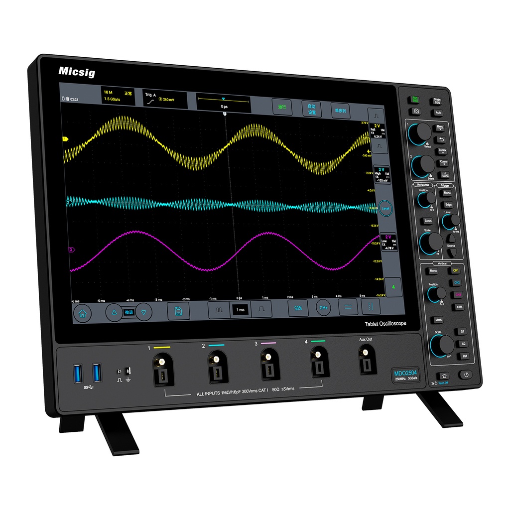
The five-times rule has a reassuring simplicity. Pick a probe with five times the bandwidth of the signal you are chasing, and the numbers on the screen look trustworthy. The moment you clip that probe onto a real node, though, the circuit sees a parallel resistance and a handful of picofarads it never asked for. A high-impedance source can sag, a fast edge can soften, and the waveform you are inspecting is no longer the waveform that was there before the probe arrived.
That gap between textbook margin and bench reality shows up in ways that are easy to misread. A resonance may shift a few megahertz, an amplifier may ring slightly, or a clock edge may lose the overshoot you were trying to capture. The five-times guideline still leaves room for loading effects because it is a bandwidth estimate, not a promise about input capacitance, ground-lead inductance, or the local impedance at the test point. Once those parasitics enter the measurement, the probe becomes part of the circuit rather than a neutral observer.
The fix is not to abandon the rule but to stop treating it as a safety certificate. At the bench, it helps to compare two probes with different loading characteristics on the same node, or to watch whether a circuit behaves differently with the probe attached. If the signal changes when the probe touches it, the five-times margin was never the whole story.
Why rise time quietly shapes what your lab can and cannot see
A scope with a sluggish rise time doesn't just blur fast edges—it quietly erases them. When the front edge of a pulse moves faster than the probe and instrument can respond, the displayed waveform becomes a smoothed approximation. That lost corner might hold the signature of a partial discharge, a metastable glitch, or a reflection that never should have been there. In effect, the lab stops seeing events that are physically present in the circuit.
Most engineers focus on bandwidth as a headline number, but rise time sets a harder limit on what actually reaches the screen. A 100 MHz oscilloscope might capture a repetitive 100 MHz sine wave, yet miss a single 3 ns transient entirely. The difference shows up in everyday work: a power rail that looks clean on the display can still be ringing at 200 MHz, and a logic signal that appears monotonic may have a runt pulse hiding in the unmeasured gap. What the instrument cannot slew fast enough to follow, it simply does not report.
Paying attention to rise time changes how a lab interprets failures. A missed trigger, an oddly stable noise floor, or a waveform that looks “too clean” often points back to insufficient edge response. By matching probe and scope rise times to the fastest edges in the system under test, the bench stops generating false confidence. The measurements remain limited, but now the limits are known—and that knowledge shapes which conclusions survive contact with reality.
Harmonics, noise, and the real cost of a front end that runs out of room
A receiver front end always looks fine on paper until a strong off-channel signal walks in and the whole chain quietly bends. Harmonics do not announce themselves as obvious distortion; they appear as faint copies of a transmitter where no transmitter should be, or as unexpected images after mixing. Noise behaves with a little more honesty, but only if there is still enough headroom left for the weak signal to rise above it. Once the gain distribution is off, the noise figure becomes a number that mainly describes what the first stage could have done under ideal conditions, not what the system actually delivers.
Running out of room is rarely a single catastrophic failure. It shows up as a slight rise in the noise floor when several carriers are present, as a wanted channel that gets spongy around the edges, or as intermodulation products that drift through the band like weather. The real expense is not just the missing signal; it is the engineering time spent chasing problems that only appear in the field, the extra filtering that should have been planned earlier, and the quieter truth that a front end designed too close to its limits will age badly as nearby services change.
There is also a practical side that data sheets do not capture. A front end with no room left cannot tolerate antenna variations, cable losses, or even a different operator on an adjacent frequency. What begins as a modest specification gap turns into a recurring support burden. The cheapest fix is usually more headroom at the start: better linearity, a lower first-stage noise contribution, and enough margin that ordinary overload events become uneventful rather than something users learn to work around.
A pre-purchase checklist that ignores brochure language and focuses on signal behavior
Most pre-purchase checklists fall apart because they repeat what a sales page already claims. Instead of circling words like “robust” or “intuitive,” pay attention to what the product does when no one is guiding the demo. Watch how it handles a slow connection, an empty search result, or a missing field. Those small, unscripted moments reveal the actual behavior you will live with.
Build your checklist around observable events rather than adjectives. Time the gap between clicking a button and getting a useful result. See whether an export opens cleanly in another tool or forces you into a workaround. Check what happens when a step fails halfway through, because that is where real software shows its character.
Treat silence as information too. If a vendor skips over setup, error recovery, or data migration, that absence usually says more than a full slide deck. A sharper checklist is not longer; it just refuses to accept brochure language as evidence.
Matching bandwidth to measurement confidence instead of chasing the highest number
It’s tempting to compare datasheet specs and assume the instrument with the highest bandwidth figure will give you the most trustworthy results. But raw bandwidth only tells part of the story. What actually matters is whether the measurement has enough confidence for the decision you’re about to make. A lower-bandwidth setup with stable, repeatable readings often beats a higher-bandwidth one that introduces noise, overshoot, or uncertainty you can’t quantify.
The real question is not “how fast can this instrument go” but “how much margin do I really need for this signal.” If your edges are slow and your tolerances are wide, pushing bandwidth higher can do more harm than good. It picks up extra high-frequency energy, amplifies jitter, and makes the trace look worse than it is. Matching bandwidth to the actual signal — not to a marketing number — keeps the measurement clean and the interpretation honest.
A practical approach is to work backward from the required rise time or the fastest edge you care about, then add only the bandwidth needed to capture it with confidence. That gives you a measurement you can defend, without chasing spec sheet bragging rights. Sometimes the best lab decision is choosing the scope or probe that’s “good enough” for the task, and using the saved attention for grounding, probing, and repeatability — the things that quietly determine whether a number can be trusted.
FAQ
Don't start with the clock frequency. A 100 MHz square wave has harmonics well beyond 100 MHz, so a 100 MHz scope rounds the edges badly. Check the rise time of the signals you actually probe. A 3.5 ns edge needs about 100 MHz of bandwidth, but a 1 ns edge is already pushing 350 MHz.
Higher bandwidth usually means a higher noise floor and more sensitivity to probing mistakes. If your probes and grounding can't keep up, the extra bandwidth mostly adds uncertainty. I'd rather put money into good probes and a slightly lower noise front end than chase a number.
It's okay for sine-like waveforms, but it breaks down on fast digital edges. Once you're looking at square waves or short pulses, edge rate is the better guide. Use 0.35 divided by rise time, then add a little margin for probe loading.
The probe can be the limiting factor before the scope is. Scope and probe bandwidth combine, and the system bandwidth ends up lower than either spec alone. A 500 MHz scope with a 500 MHz probe gives you roughly 350 MHz of usable system bandwidth, so plan both together.
Enough to cover your fastest expected edge, not double the clock just for comfort. If you're already near the limit of a 200 MHz scope on current projects, a 350 MHz or 500 MHz scope makes sense. If not, extra headroom may just sit unused while you deal with more probe noise.
Feed a known fast edge into the scope with a direct BNC connection and note the rise time. Then repeat with your usual probe. If the probe makes the edge notably slower, your probe is the bottleneck. If the direct connection is already slow, the scope is limiting the measurement.
Yes, sometimes in opposite directions. Analog work often rewards extra bandwidth for amplitude accuracy, but noise can become a problem. Digital work depends more on clean edge capture and timing, so a fast front end with good sample rate can beat a high bandwidth badge on a sluggish scope.
Conclusion
A useful bandwidth decision starts with the fastest edge your probe actually touches, not the number printed on a scope or its price tag. Labs often default to the five-times rule and then wonder why a 100 MHz clock looks rounded once a passive probe loads the node. The more honest question is whether the instrument can follow the rise time that matters for your work. If the front end rolls off before that edge, you lose the very detail that separates a clean validation from a guess, regardless of how much bandwidth the datasheet claims.
What really limits a lab is rarely the headline bandwidth; it is how the front end behaves when harmonics, noise, and fast transitions arrive together. A scope with no headroom turns a modest overshoot into an artifact you might chase for days. Before buying, ignore brochure language and build a short checklist around real signal behavior: probe loading, edge speed, required harmonic content, and the confidence you need in a measurement. Choosing a scope then becomes a conversation about evidence, not a race to the highest number on the front panel.
Contact Us
Contact Person: Lily
Email: [email protected]
Tel/WhatsApp: +49 (0) 2161 49526-0
Website: https://tps-elektronik.com/en/